
Dynamic Time Warping Algorithm for trajectories similarity
The Dynamic Time Warping (DTW) algorithm is one of the most used algorithm to find similarities between two time series. Its goal is to find the optimal global alignment between two time series by exploiting temporal distortions between them. DTW algorithm has been first used to match signals in speech recognition and music retrieval\(^1\). However, its scope of use is wider as it can be used in Time series of two-dimensional space to model trajectories. In the case of modeling and analyzing trajectories, the DTW algorithm stands out as a good way of computing similarity between trajectories.
A time series is a serie of data points indexed (or listed or graphed) in time order. Most commonly, a time series > is a sequence taken at successive equally spaced points in time.
In this article, we implement the DTW algorithm for human mobility analysis to find similarities between trajectories.
Quick reminder: A spatial trajectory is a sequence of points \(S = (…, sᵢ, …)\) where sᵢ is a tuple of longitude-latitude such as sᵢ = (φⱼ, λᵢ). We denote the trajectory length by \(n\) = |S|. We denote a subtrajectory of S as \(S(i, ie) = S[i..ie]\), where \(0 ≤ i < iₑ ≤ n - 1\). The identified pair of subtrajectories is called a motif.
We can extract trajectories from several data sources. Some of the data sources used for capturing human mobility traces are as follows.
- Call Detail Records (CDRs). Mostly accessible by network operators, CDRs have the advantage of having a huge sample size due to the ubiquity of mobile phones. These datasets offer a tower level precision and for obvious privacy reasons, these datasets are not publicly available.
- Location-Based Social Network (LBSN). With the increasing use of social networks, new sources of data have emerged. Social Network platforms like Facebook, Twitter or FourSquare provide geographic check-ins or geolocated publications. These data, mostly freely available, can be used as a basis to model human mobility trajectories. The main drawback of LBSN's dataset is the sparsity of the location, indeed, entries are set only when check-ins are made.
- GPS data. Compared to the data sources previously cited, GPS data offers high spatial and temporal precision and offer a good socle to analyze full trajectories such as car movements, people movements,… The drawback of GPS data is that it requires additional preprocessing due to errors when the GPS signal is noisy.
To implement the DTW algorithm, we can either use an LBSN dataset or raw GPS data. In our case, we need accurate location data to draw trajectories, so we are going to use a GPS dataset. Many GPS datasets are available freely on the internet. Most of these datasets are designed from real-world data collected over a period of time. As example, we have the popular Nokia and Geolife datasets.
Definitions
A time series is a serie of data points indexed (or listed or graphed) in time order. Most commonly, a time series is a sequence taken at successive equally spaced points in time.
A spatial trajectory is a sequence of points \(S = (…, sᵢ, …)\) where sᵢ is a tuple of longitude-latitude such as sᵢ = (φⱼ, λᵢ). In the GIS world, a trajectory is represented as a LineString associated witht an attribute of time.
We denote the trajectory length by \(n\) = |S|.
We denote a subtrajectory of S as \(S(i, ie) = S[i..ie]\), where \(0 ≤ i < iₑ ≤ n - 1\). The identified pair of subtrajectories is called a motif.
In the language of GIS, therefore, a trajectory is represented as a LINESTRING feature together with an attribute representing time.
To implement the DTW algorithm, we can either use an LBSN dataset or raw GPS data. In our case, we need accurate locations to draw trajectories, so we are going to use a GPS dataset. Many GPS datasets are available freely on the internet. Most of these datasets were built from real-life data collected over a period of time. As example, we have the popular Nokia and Geolife datasets. The drawback of these datasets is their sparsity and size. The goal of this blogpost been to implement the DTW on two sub-trajectories, discovering a motif is not a priority.
For the testing purposes, we can use a sample of the Geolife dataset which contains trajectories of 182 individuals collected during 3 years by a research team of Microsoft Research Asia. It has a total of 17,621 trajectories of about 1.2 million kilometres.
To analyze this sample dataset, we can use the Pandas library on Python. To better understand how a trajectory similarity algorithm works, we will compute the distance manually using the DTW algorithm.
Requirements:
- Python ≥3.6
- Pandas library
- Geolife sample dataset, available on this link.
- Some motivation and a big smile 😃
Let's set up the tools and explore our dataset:
import pandas as pd
import copy
import matplotlib.pyplot as plt
from numpy.random import normal

file = "geolife_sample.txt.gz"

df = pd.read_csv(file, sep=',')
df.sort_values(by=["uid"], inplace=True)

df.head()
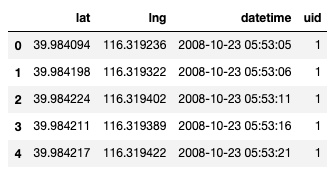
As you can see on figure 1, we have 4 main attributes in our dataset: lat (latitude), lng(longitude), datetime and uid(User ID). The coordinates are expressed in decimal degree using the WGS84 datum.
To compute the DTW, we will extract sub-trajectories of 2 users, namely u₁ and u₂. The identified pair of sub-trajectories is called a motif. To find a motif with the closest distance between two sub-trajectories, a straightforward approach is to compute recursively the distance between the trajectories and to keep the trajectories that meet a particular threshold.
Depending on the complexity of the technique used and on the size of the dataset, this operation can quickly escalate into a lengthy process.
The main goal of this article is to guide through the process of finding the similarity between two trajectories and to find the warp path between two time series that is optimal.
In order to find the similarity between two trajectories, we need to compute a distance matrix dG which can be considered as a multidimensional array mapping every point of a trajectory P with points of a trajectory Q by their real distance. To find the distance between two geographic points, we can use the Harvesine formula illustrated in the equation below:
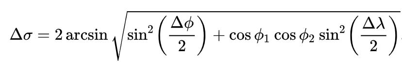
where λ₁, ϕ₁ and λ₂, ϕ₂ are the geographical longitude and latitude in radians of the two points 1 and 2, Δλ, Δϕ be their absolute differences\(^2\).
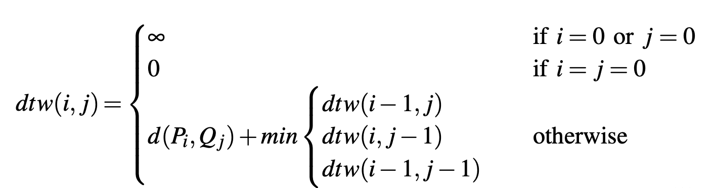
To compute the distance between u1 and u2 using DTW, we can define a function distance that computes the ground distance between two points. Then by using the principle of dynamic programming, we can go through the matrix recursively until we get the final score which will represent the DTW between our two trajectories.
The equation to compute the DTW P and Q (respectively u1 and u2) is the following:
Let’s implement the algorithm in Python. We will structure our code by using classes.
First, we have to create a class that we are going to use. The first class should define a point, represented by longitude, latitude and a timestamp.
class Point:
	def __init__(self, latitude, longitude):
		self.latitude = latitude
		self.longitude = longitude

	def __str__(self):
		return "Point("+self.latitude+", "+self.longitude+")"
Then, we can declare a class representing trajectories:
class Trajectory:
    def __init__(self, points = []):
        self.points = points
We will create a function that takes a point as input and returns the ground distance between the initial point (defined by self) and the point added as parameter.
def getDistance(self, point2):
        delta_lambda = math.radians(point2.latitude - self.latitude)
        delta_phi = math.radians(point2.longitude - self.longitude)
        a = math.sin(delta_lambda / 2) * math.sin(delta_lambda / 2) + math.cos(math.radians(self.latitude)) \
        * math.cos(math.radians(point2.latitude)) * math.sin(delta_phi / 2) * math.sin(delta_phi / 2)
        c = 2 * math.atan2(math.sqrt(a), math.sqrt(1 - a))
        distance = cls.R * c
        return distance
Now, we have all the prerequisites to implement the code and find the distance between two trajectories. With our minimalist code, we can represent a trajectory as a list of Point[]. We can represent the ground distance between trajectories in a matrix.
We can use the following code to parse the geolife sample dataset to extract the two trajectories:
# Here, we get the unique trajectories
unique_uids = df.drop_duplicates(["uid"])
unique_uids = unique_uids["uid"].to_list()

# Then, we split the trajectories
points = []
trajectories = []
for i in range(len(unique_uids)):
    tmp_df = df.loc[df["uid"]==unique_uids[i]]
    len(tmp_df)
    for j in range(len(tmp_df)):
        points.append(Point(tmp_df.iloc[j][0], tmp_df.iloc[j][1], tmp_df.iloc[j][2]))
    trajectories.append(copy.deepcopy(points))
    points.clear()
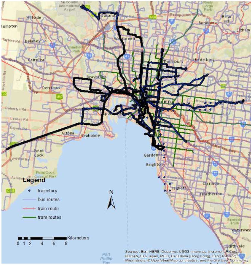
The trajectories are now stored in a list called trajectories. After executing this code, you can see that we obtain 2 trajectories from the dataset.
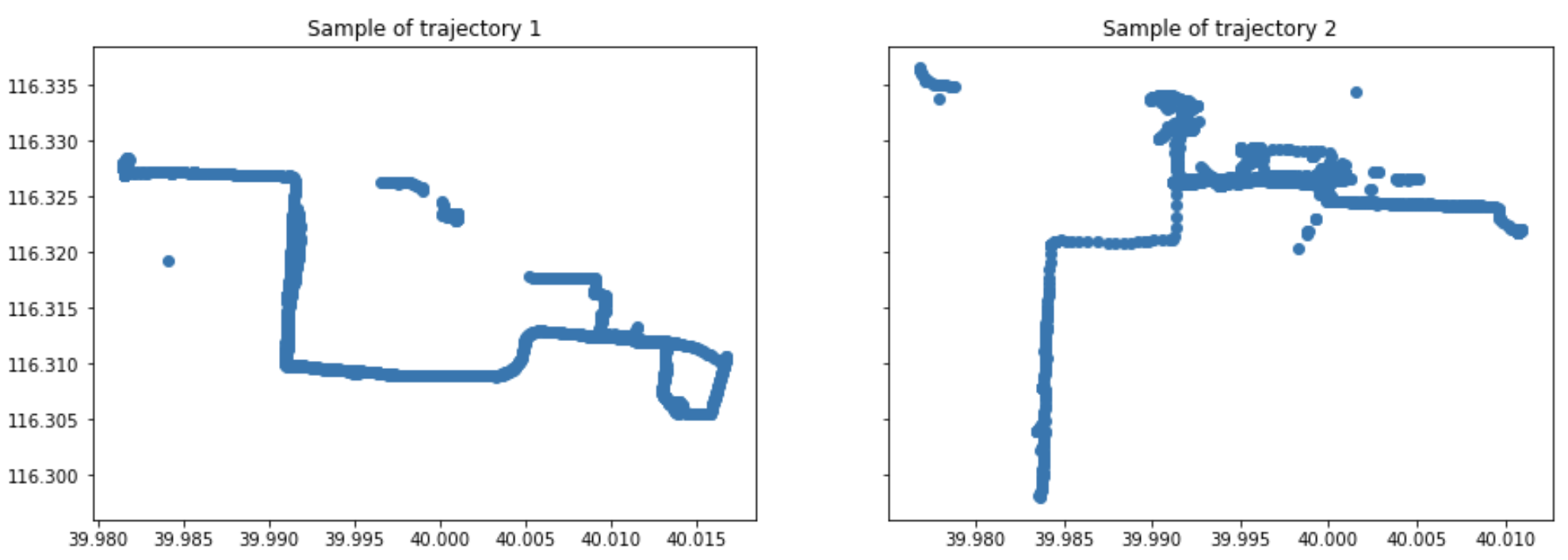
As you can see in the figure above, the two trajectories are quite dissimilar, finding the optimal match using DTW gives no real interest in this case. For a sake of simplicity, we generate a new trajectory based on an existing one by adding some Gaussian noise.
To achieve that, we just add a new method in the Trajectory’s class:
def addNoise(self, mu, sigma):
        return Trajectory([Point(i.latitude + normal(mu, sigma), i.longitude + normal(mu, sigma), i.t) for i in self.points])
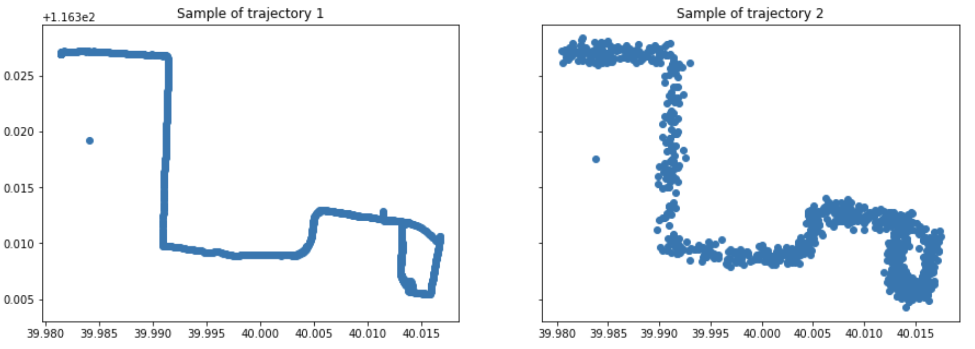
Now, we can use the first trajectory from the dataset a reference, we call it P, and we create a second trajectory Q based on P by using the method addNoise.
P = Trajectory(trajectories[0])
Q = P.addNoise(0, 0.0005)
Warping function
The warping function is a function that minimizes the total distance between the points of the two given trajectories. Before defining the warping function, we will create a distance matrix between the two trajectories using the following code:
row = []
matrix = []
for i in Q.points:
    for j in P.points:
        row.append(round(i.getDistance(j), 2))
    matrix.append(row)
    row = []
The table below shows a sample of the distance matrix between the ten first points of P and Q.
| 0.06 | 0.05 | 0.05 | 0.05 | 0.06 | 0.06 | 0.07 | 0.07 | 0.07 | 0.07 |
| 0.07 | 0.06 | 0.05 | 0.04 | 0.04 | 0.04 | 0.04 | 0.04 | 0.04 | 0.04 |
| 0.12 | 0.11 | 0.1 | 0.09 | 0.08 | 0.07 | 0.06 | 0.06 | 0.06 | 0.06 |
| 0.05 | 0.04 | 0.03 | 0.03 | 0.02 | 0.03 | 0.04 | 0.04 | 0.04 | 0.04 |
| 0.1 | 0.09 | 0.08 | 0.07 | 0.06 | 0.05 | 0.04 | 0.04 | 0.04 | 0.04 |
| 0.12 | 0.1 | 0.09 | 0.08 | 0.07 | 0.05 | 0.04 | 0.04 | 0.04 | 0.04 |
| 0.12 | 0.11 | 0.1 | 0.09 | 0.07 | 0.06 | 0.05 | 0.05 | 0.05 | 0.05 |
| 0.06 | 0.05 | 0.04 | 0.03 | 0.01 | 0.0 | 0.02 | 0.02 | 0.02 | 0.01 |
| 0.12 | 0.1 | 0.09 | 0.08 | 0.06 | 0.05 | 0.04 | 0.04 | 0.04 | 0.04 |
| 0.21 | 0.19 | 0.18 | 0.17 | 0.16 | 0.14 | 0.13 | 0.13 | 0.13 | 0.13 |
After building our distance matrix, we can now define a warping function that will be used to find the optimal warping path in the whole distance matrix. The warping function should take as input the accumulated distance matrix and should return a list of index pairs representing the optimal warping path.
def warping_path(D):
    n = D.shape[0] - 1
    m = D.shape[1] - 1
    P = [(n, m)]
    while n > 0 or m > 0:
        if n == 0:
            min_val = (0, m - 1)
        elif m == 0:
            min_val = (n - 1, 0)
        else:
            val = min(D[n-1, m-1], D[n-1, m], D[n, m-1])
            if val == D[n-1, m-1]:
                min_val = (n-1, m-1)
            elif val == D[n-1, m]:
                min_val = (n-1, m)
            else:
                min_val = (n, m-1)
        P.append(min_val)
        (n, m) = min_val
    P.reverse()
    return np.array(P)
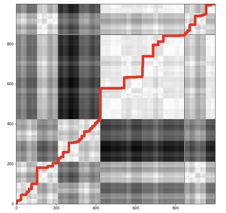
For simplicity, we can illustrate the distance matrix as a confusion matrix where the darker cells represent high values while the lighter ones represent small values. Figure 3 shows the optimal warping path along the distance matrix between trajectories P and Q.
Time complexity
For two trajectories N and M, the time complexity of the DTW algorithm can be presented as O(N M). Assuming that |N|>|M|, the time complexity is determined by the highest time spent to find the distance between the two trajectories, so in this case, time complexity of the algorithm will be O(N²).
DTW algorithm is known to have a quadratic time complexity that limits its use to only small time series data sets\(^3\).
Drawbacks of DTW
DTW performs well for finding similarity between two trajectories if they are similar in most parts, but the main drawback of this algorithm is that DTW is sensitive to noise i.e. it gives non-meaningful results when it comes to comparing two trajectories containing significant dissimilar portions. Another drawback is the time complexity which can be a bottleneck for finding similarities in large datasets. Some techniques based on DTW have been developped to tackle this problem. Some of the most popular techniques are PruneDTW, SparseDTW, FastDTW and MultiscaledDTW. These techniques are not covered in this article.
Other similarities measures
By matching each point of a trajectory to another, DTW algorithm gives good results with uniformly sampled trajectories. Meanwhile, with non-uniformly sampled trajectories, DTW adds up all distances between matched pairs\(^3\).
Algorithms available for finding similarities between trajectories can be sorted by applying a trade-off between efficiency and effectiveness. Among the most efficient method in terms of performance, the Euclidean Distance ranks amongst the best. In fact, Euclidean Distance between two time series is simply the sum of the squared distances from \(n^{th}\) point to the other. For comparing trajectories, Euclidean distance shows a great performance in terms of computational time, but its main disadvantage for time series data is that its results are very unintuitive. It is also interesting to explore some similarity techniques for text that can be transpose to trajectories. Among those techniques, we have techniques based on Edit-distance like LCSS (Longest Common Subsequence), EDR (Edit Distance of Real Sequence), ERP (Edit Distance with Real Penalty), TWED (Time Warp Edit Distance) and EDwP (Edit Distance with Projections).
You can find the source code of our experiments on this repository.
References
- Lijffijt, J., Papapetrou, P., Hollmén, J., & Athitsos, V. (2010, June). Benchmarking dynamic time warping for music retrieval. In Proceedings of the 3rd international conference on pervasive technologies related to assistive environments (pp. 1-7).
- https://en.wikipedia.org/wiki/Haversine_formula
- Salvador, S., & Chan, P. (2007). Toward accurate dynamic time warping in linear time and space. Intelligent Data Analysis, 11(5), 561–580.